This post aims to explain the workings of self and multi-headed attention.
Self-Attention
Self-attention is a small part in the encoder and decoder block. The purpose is to focus on important words. In the encoder block, it is used together with a feedforward neural network.
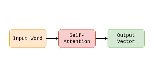
Zooming into the self-attention section, these are the major processes.
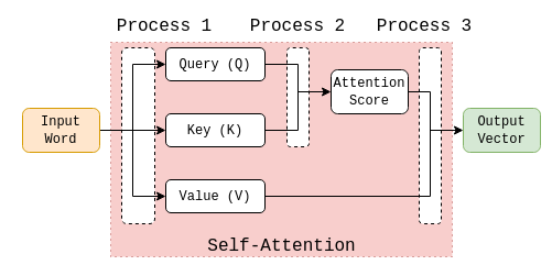
Process 1 - Word embedding to Query, Key and Value
There are three key parameters introduced in this concept—query, key and value. To avoid confusion, I will use Q, K and V to reference them.
These vectors are calculated from the word embedding. Another way to understand this process is the input embedding is translated into three different versions of itself, from embedding space to Q, K and V subspace.
This is done by projecting the input to three different sets of weights, i.e. Query weight, Key weight and Value weight. All weights act as a projection medium which is trainable.
Each word in the sequence will have their query, key and value.
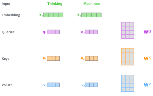
Image Source: jalammar.github.io
One thing to note is all three values mean nothing. They are just mathematical representations of the input word in different vector subspace which can be used for calculations. That’s it.
Process 2 - Calculating Attention Score
Up to here, the input embedding has been projected to Q, K and V subspaces. In this process, Q and K are used for calculating the attention score.
Let’s say we want to encode eat from the sentence They eat fried noodles, after process 1, all input words will have Q, K and V as below.
Note: Starting from here, all examples are referring to the process of one word only. In a real application, every word will have to go through these steps.
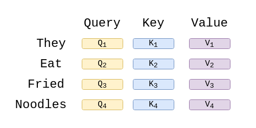
In process 2, the scores are calculated by performing dot products of Q of eat with transposed K of every word in the sequence, including itself. The result for a single word is a vector of size (1, 4) which holds the value of every dot product result.
The size (1, 4) is used as an example in this post for simplicity. (1, 4) means a word has 4 embedding length(or features).
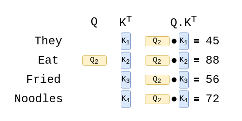
Then, every score is divided by 8. According to this source, “This leads to having more stable gradients” source.
score = [32, 88, 56, 72]

after divide by 8
score = [4, 11, 7, 9]
The attention score is calculated by applying the softmax function to all values in the vector.
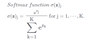
This will adjust the scores so that the total will add up to 1.
Softmax result

softmax_score = [0.0008, 0.87, 0.015, 0.011]
The attention scores indicate the importance of the word in the context of word being encoded, which is eat. Higher value, higher importance.
Process 3 - Calculating Output Vector
The last process is to produce the output vector. Up to here, we have the attention score and V.
Here, the softmax scores are multiplied to their respective V. Then, the values are added together to produce the output vector.
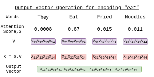
For example, to produce value for eat with respect to they the calculation is
softmax score: 0.0008
V for "they" = [V11 V12 V13 V14]

The Multiplication values, X are:

X = [X11 X12 X13 X14]
X = [0.0008(V11) 0.0008(V12) 0.0008(V13) 0.0008(V14)]
The green box is the output vector of self-attention section. This is the value that is passed to the next part of the block.
How Matrix Transform at every Process
Before we go to the multi-head, let us understand the transformation of matrixes by observing the dimension at every process. I am using the dimensions from the transformer model.
According to the paper, the model requires input dimension to be (1, 512) for a single word vector.
For our example sentence, The matrix size will be (4, 512). As the value passing through every parts of the encoders and decoders, the embedding size(or number of features) will stay constant at 512.
That means, the input and output matrix that pass through self-attention has matrix of size (4, 512).
Evaluating self-attention
Let’s revisit the self-attention process.
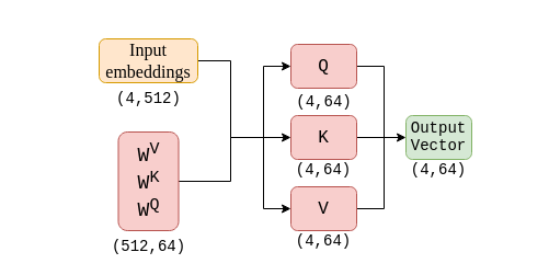
If we look at the output of self-attention, the size of the output matrix is not equal to the input. This is anticipated as self-attention is to be used as one of the many heads of the multi-headed attention.
Multi-head Attention
As said before, the self-attention is used as one of the heads of the multi-headed. Each head performs their self-attention process, which means, they have separate Q, K and V and also have different output vector of size (4, 64) in our example.
To produce the required output vector with the correct dimension of (4, 512), all heads will combine their output by concatenating with each other.
Assume h1, h2 and h3 are the outputs from 3 different heads.
h1 =    [1, 2, 3]
        [4, 5, 6]
        [7, 8, 9]

h2 =    [10, 11, 12]
        [13, 14, 15]
        [16, 17, 18]

h3 =    [19, 20, 21]
        [22, 23, 24]
        [25, 26, 27]

h_concatenate = [1, 2, 3, 10, 11, 12, 19, 20, 21]
                [4, 5, 6, 13, 14, 15, 22, 23, 24]
                [7, 8, 9, 16, 17, 18, 25, 26, 27]
So you can view the whole process this way.
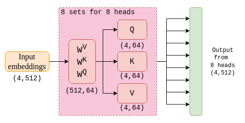
To produce the output, the combined output is multiplied with the output projection matrix.
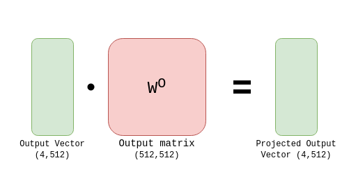
This is the output for the multi-headed attention layer, which is used for the next stage.
Multi-head attention in Decoder
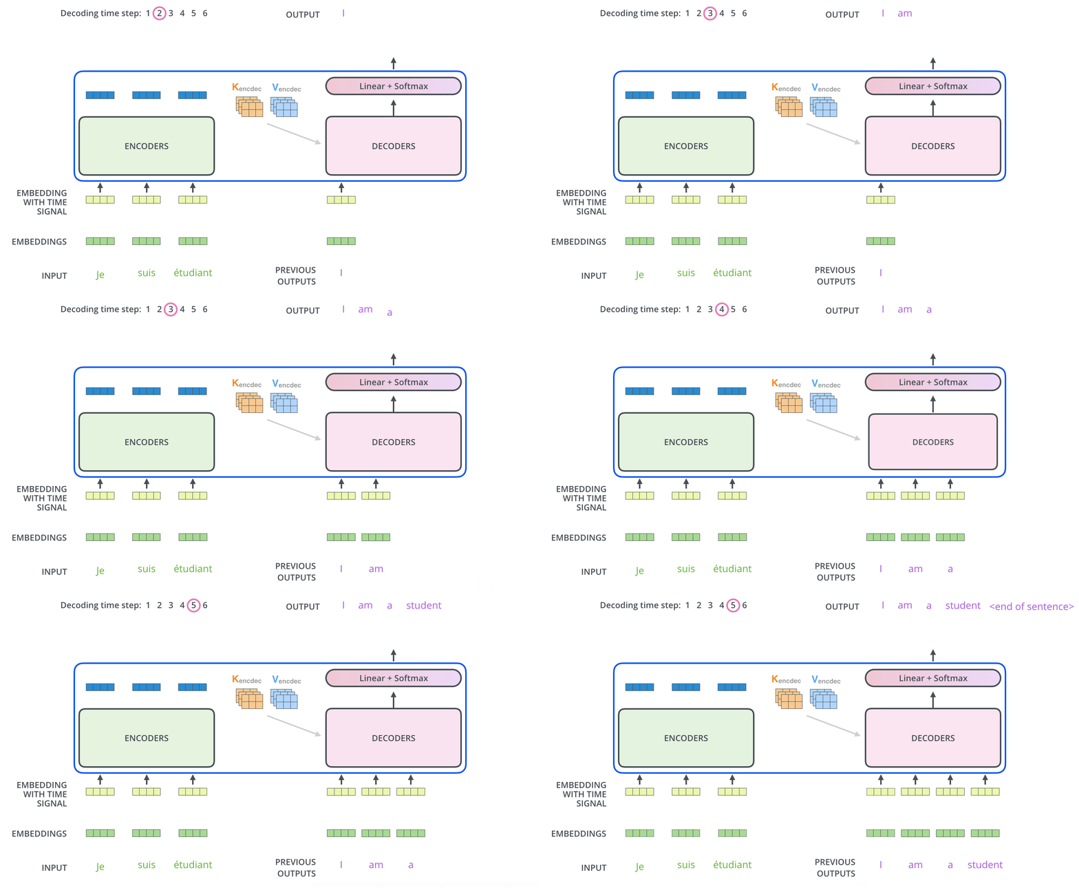
The output of encoder stack will produce K and V for the input sequence. This is then pass to the Decoder section.
In the decoder, the Self-attention section does not compute the K and V from the sequence to be decoded. Instead, it only compute Q and used K and V from the encoder stack.
This is how the two sequences are related.
Conclusion
I hope you have good insights regarding self-attention algorithms. The example given is using the transformer parameters value. The differences compared to BERT are:
- Embedding Dimensions
Transformers = 512 BERT = 768 - Number of heads
Transformer = 8
BERT = 12
And of course, BERT is and encoder only model while Transformer is both encoder and decoder. Thanks for reading. Have a nice day!